Stam solver working
This week I worked hard on getting the fluid solver in the style of Jos Stam working. The basics were easy enough, but Stam makes some simplifying assumptions, so the continuation was not quite trivial. But combined with what I learned in my earlier work on the free-surface simulator, I managed to put together a fast, stable, flexible and pretty fluid solver that I’m more than a little proud of.
Fast? Yes: in contrast with my previous solver, this one is not bound by the CFL condition. That means that it does not need very small timesteps, so it can simply step at 1/60 second instead of 1/1000. The tradeoff here is that it is less physically accurate, since it violates the law of conservation of momentum — but it’s a game, who cares? Not only is the time step larger, but we can do more of them per second; on my GeForce 9800 GT, it can maintain a framerate of 700 fps. And that is with a 256x256 grid: sixteen times as many pixels as my previous solver! It should be sufficient to make it still pull those 60 fps on older hardware.
Stable? Yes: I can apply accelerations of up to 100 screens per second squared, resulting in velocities of several screens per second, and the simulation still looks smooth. That is fast enough to send any poor jellyfish player slamming into a wall. Moreover, larger velocities simply result in some artifacts; they do not cause the entire simulation to blow up.
Flexible? Yes: whereas Stam assumes that the fluid is in a rectangular box, I added more general boundary conditions. I can now place walls into the fluid and have the flow go nicely around them. Although only rectangles are supported by the data structures at the moment, the fluid simulator itself accepts any grid of boolean (wall/fluid) values for the walls in the level. This is one of the places where I made a significant improvement to Stam’s algorithms based on my previous experience. For the boundary conditions, Stam loops over the wall cells and copies values from outside the walls. These values inside the walls can then be read by subsequent steps, which do not have to care that they come from inside the wall. Instead, I keep an array of 4 coefficients for each cell, corresponding to the 4 neighbouring cells. Coefficients for wall neighbours are 0. Each access to a neighbour’s value is multiplied by its coefficient, so if there are nonsense values in the wall cells, no-one will know! This saves many passes over the array to satisfy the boundary conditions.
Pretty? Yes, pretty too! Apart from the velocity field moving along itself, I also added a colour field moving along the velocity field. I added some code for colour injectors, so we can have “ink” leaking into the fluid to trace its movement. It’s not really ink, because I use additive blending instead of multiplicative; it’s actually more like tonic under blacklight. I plan to have sparkles later on, but I think I’ll keep this too:
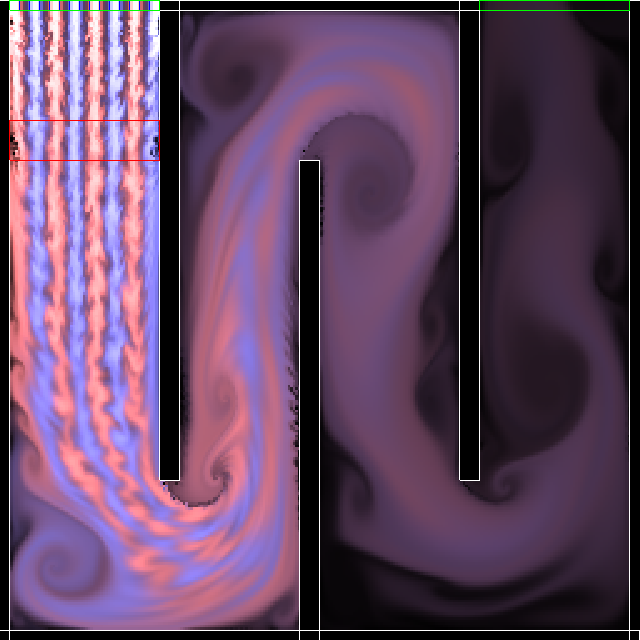
At the top left are eight colour injectors with alternating blue and pink colours. Around them, and at the top right as well, you see a green box, which represents an inflow/outflow. These are connected to some nonexistent “outside world” where the pressure is 0. The red box represents a force, which accelerates the fluid downwards. The black boxes outlined in white are, obviously, walls. You can see the fluid nicely flowing through the tunnel, creating many gorgeous vortices around the corners. Seeing it in motion is even better!