Around The World, Part 7: Temperature and rain
This post is part of a series about Around The World, a game of exploration and discovery at sea. The game is currently in early development. If you're new to this project, you can read up on it here.
We now have prevailing wind patterns going, so it’s time to turn to the other two important parameters that define the weather: rain and temperature.
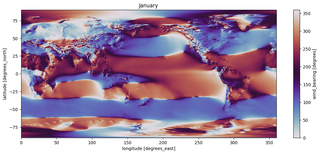
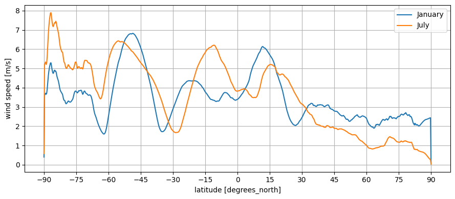
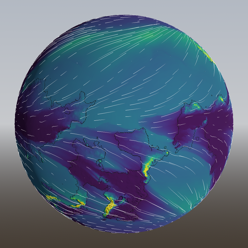
During a sleepless night, I got a bit overboard and wrote an analysis over 10 years of actual weather data from Earth, using the ERA5 data set. That led me to tweak the wind a bit as well, based on pretty maps and plots like these:
You can view the notebook on GitHub including instructions on how to run it yourself (warning: 34 GB download needed).
Is it getting hot in here?
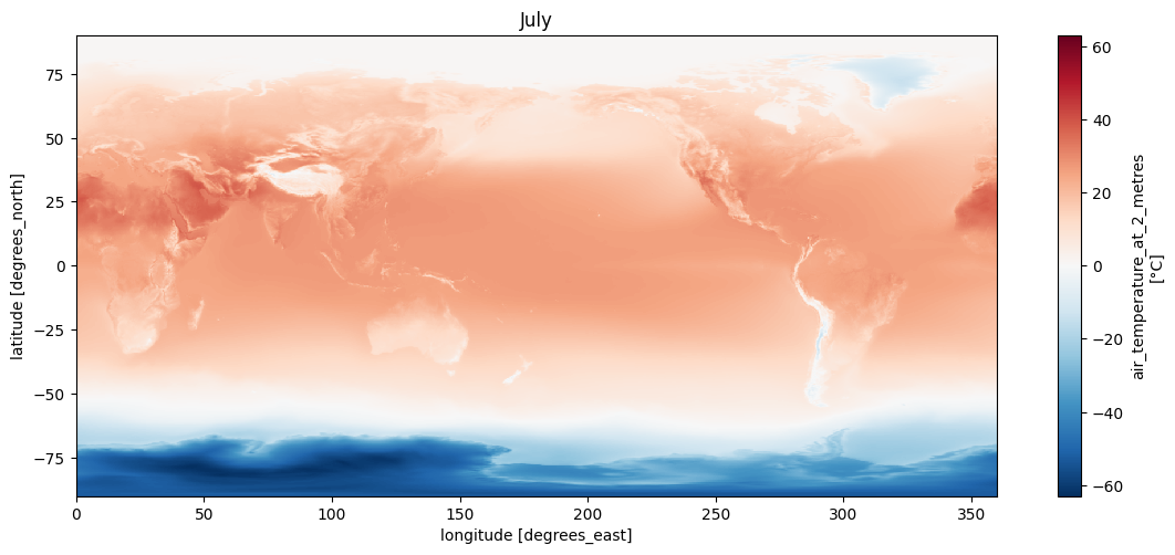
Let’s tackle temperature first, because it’s easiest. My analysis of Earth temperature has already been split into January and July to account for seasonal variation, but we’re aiming for a yearly average at the moment. As it turns out, temperature depends primarily on latitude:
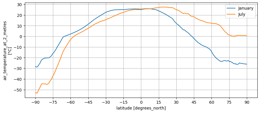
You can see that seasonal variation is higher in the norther hemisphere, because that’s where most landmasses are, and also that temperature is generally higher there for the same reason. But we’ll ignore that for the moment.
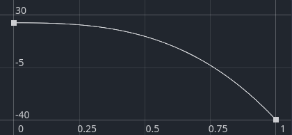
We can implement this as a curve, where the x axis is the absolute latitude divided by 90 degrees, and the y axis is the temperature in degrees Celcius:
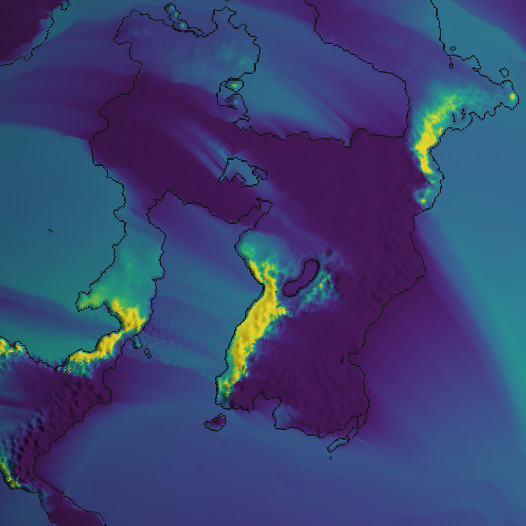
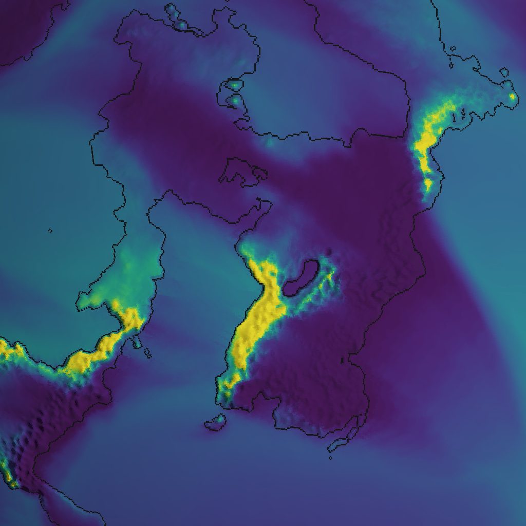
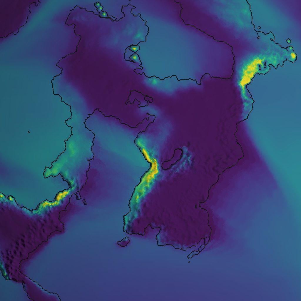
Temperature also varies strongly by altitude. You can clearly spot the mountain ranges and Tibetan plateau, where it’s around the freezing point even in the middle of summer:
As a rule of thumb, temperature decreases by 6.5 °C per kilometer of altitude. We have a height map, so that’s easy to implement.
To make things not perfectly smooth, of course we add some simplex noise. And those three factors taken together gets us this:
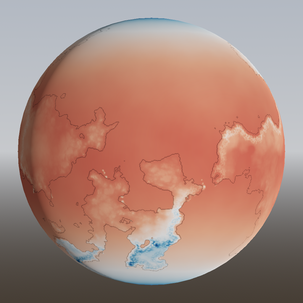
I think that looks just fine for now! It may seem like the polar regions are too small compared to the Earth image above, but that’s a trick of perspective. The temperature crosses the 0 °C threshold around 60 degrees of latitude in both cases.
Hallelujah, it’s raining
Where temperature was very straightforward, precipitation (I’ll call it rain from now on) is a lot harder, because it’s strongly dependent on wind. Like with temperature, we’re not yet concerned with seasonal variations; we just want to compute yearly rainfall for each location.
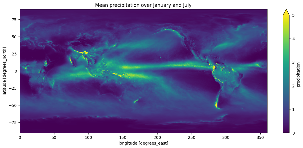
For comparison, here’s a map of rainfall on Earth which (spoiler alert) we won’t be replicating perfectly today:
Rain is produced by airborne moisture. Airborne moisture is produced by evaporation of water from the surface. In my model, evaporation only happens over water. In reality it happens over land too, but the amount of evaporation depends on how wet the land is, which depends on how much rain fell there, which is what we’re trying to find out in the first place. Chicken and egg.
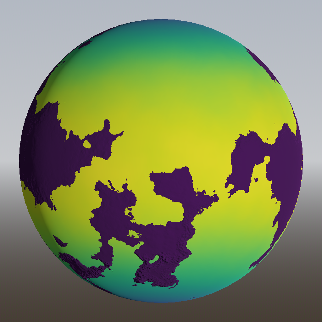
And of course evaporation depends on temperature. I couldn’t find a good reference to tell me how to map temperature to evaporation, so I created a curve by just eyeballing it. Here’s the evaporation map, with the same colour ramp as the Earth map above:
Conceptually, the algorithm lifts all this moisture into the air at once. Then it starts moving it around in discrete time steps, following the prevailing winds that we created previously. This is an advection process, so I’m using the “backwards advection” technique from the previously mentioned paper by Jos Stam. For each grid cell, we take a step backwards along the velocity. At the point where we end up, we linearly interpolate the current airborne moisture between the four nearest grid cells. This becomes the airborne moisture in our current grid cell. The advantage of this approach (apart from numerical stability) is that it’s easy to run it in parallel on multiple CPU cores, unlike forward advection methods, which might need to perform concurrent writes.
Now that we have moving moisture, where does it fall? Again I failed to find definitive numbers or formulas, but what everyone else seems to be doing (for h in hexes:, Here Dragons Abound, Undiscovered Worlds) is making it rain a little whenever there is moisture in the air at all, and a lot if the wind blows uphill. The latter effect happens because the air is forced upwards, reducing pressure and causing the air to expand, which causes it to cool down, and cold air can’t contain as much moisture. This is the cause of rain shadows behind mountains: the air coming over the mountains has already lost all its moisture on the way up, so the region behind the mountain range is quite dry.
If my understanding is correct, then we don’t need to look at altitudes and slopes at all; we can simply look at the local temperature, which is already decreasing the higher up we go. And this should automatically take care of increased rainfall in colder regions as well.
My model is very simple: every time step, after moving the moisture around, a fraction of the moisture will fall in its current location as rain. What fraction that is, depends on the temperature via a curve that I can manually control.
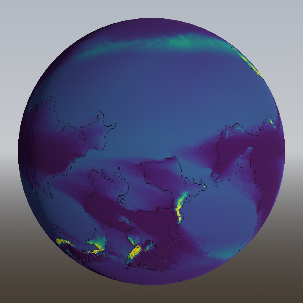
We run this for a fixed number of time steps (I’m using 100 here) and that gives us this:
You can clearly see that a lot of rain is falling in the mountains, and that the land behind it is much drier. There’s also a band of rain around the pole, which is around 50 degrees latitude. This is probably some kind of interaction between the evaporation and precipitation curves, but such bands seem to occur in real life too, albeit for entirely different reasons.
However, I’m not satisfied, and you can see why if we zoom in:
There are very straight and unnatural streamlines visible. These are caused by the fact that we use only our prevailing wind, which is constant over time.
Moreover, there are some strange ridge-like artifacts in some places, which are caused by the fact that we use a fixed time step. They could be eliminated by using smaller time steps, but then the algorithm would run even slower than it already does (more about that later).
We can fix both problems by introducing… you guessed it… simplex noise. During the advection step, we add some noise to the wind vector. And the seed of this noise is changed in every time step, so it doesn’t sample from the exact same location every time.
This almost entirely gets rid of the artifacts and makes things look pleasantly organic:
There appears to be some rainfall directly behind the mountains, which is not realistic. It’s around -10 °C in these mountains, and our curve specifies that we lose around 30% of moisture at that temperature. Let’s bump that up a bit:
Much better. This shows the usefulness of just faking things, rather than simulating them; it gives you full control in case you need it.
Quickly now
The entire world generation process will run at the start of each game, and possibly whenever the player loads a game too. It’s not nice to make them wait for a long time. I decided that on slow hardware, the wait should be at most 30 seconds. But I have fast hardware, so on my computer, it should be at most 5 seconds. Before rain generation, we had about 2.5 seconds of that budget left. To leave some headroom for future additions, I’d like rain generation to take no more than 1 second.
But it currently takes 15 seconds. Oops.
What can we do?
First, there’s some low-hanging fruit. I mentioned before that I run most algorithms in parallel over each of the 6 cube faces, and that includes rain. My CPU has 24 cores, so three quarters of those will be sitting idle during that time. The solution is simple: split each cube face into more parts, so that all cores can be fully utilized. This could theoretically give a 4× speedup, but in practice gave me only 2.2×, perhaps because there’s some other bottleneck now like memory bandwidth. We’re now down to 6.9 seconds.
Fusing some loops got it down to 6.3 seconds, but that’s still way too much.
If I turn off the simplex noise (which, remember, is generated anew for every time step), the straight lines and artifacts come back, but running time goes down to 2.5 seconds. Removing the noise is not an option, but maybe we can do something smarter than generating new noise for every time step? So I tried generating two different noise fields and alternating between them. That wasn’t enough, but with five noise fields (instead of 100, remember), it runs in 2.7 seconds and the result looks almost identical to what we had before:
Next up is to do something about those 100 time steps. After that time, 99.98% of moisture has dropped from the air. But we don’t need this to be perfectly moisture-preserving! All we need is that wind moving inland gets enough chance to drop almost all of its moisture, and then we can stop the process because the situation is pretty much stable.
With the right time step size, I was able to dial down the number of steps to 50 with hardly any visible impact. Over 95% of moisture is still dropped with this configuration, and the algorithm runs in 1.5 seconds. (I could of course make the algorithm abort automatically as soon as some fixed percentage of moisture has been dropped, but then I lose control over the exact running time. It’s a tradeoff.)
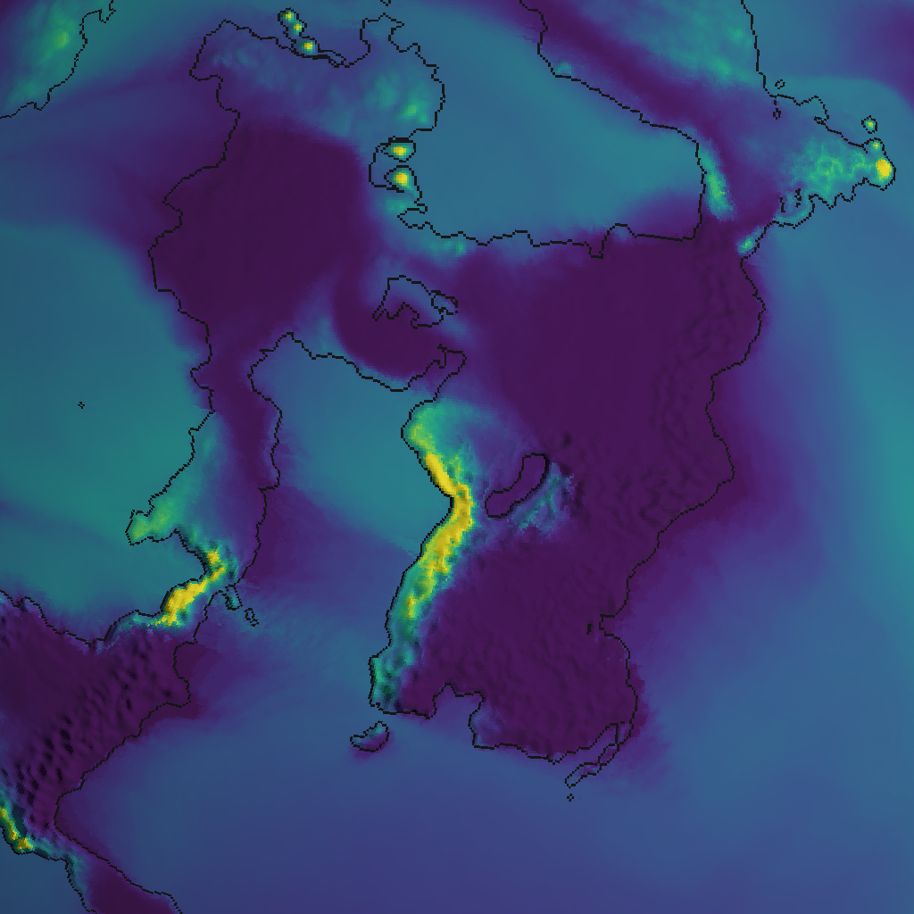
With an even bigger time step, the artifacts become too obvious. Counteracting them with stronger simplex noise isn’t feasible, because it tends to blur the precipitation map too much, especially around mountains. So I came up with another hack: make the amount of noise dependent on temperature. At lower temperatures, there’s a lot of rainfall, so we care a lot about the exact place where it drops. But at higher temperatures, there’s less rain, so we can get away with more noise and blurring. And that lets me increase the time step size even more, which lets me reduce the number of time steps to 25. Running time is now 0.96 seconds, and I’m calling that a success. Here’s the resulting rain map:
Now that we know the local climate at each point in our world, we can decide what vegetation we would expect there. But that’s for the next post!