Around The World, Part 8: Seasons
This post is part of a series about Around The World, a game of exploration and discovery at sea. The game is currently in early development. If you're new to this project, you can read up on it here.
In the last post, we developed some basic but useful algorithms to generate temperature and rain maps for an entire year. However, these assumed that the weather is constant throughout the year. As any citizen of Earth knows, that is not quite true, so let’s fix it!
Two weathers
I don’t want to create an entire weather simulation in the game, so we’re once more going to fake it. Instead of coming up with one fixed weather pattern, we’ll create two: one in January, one in July. These are assumed to cover the extremes in each location. (The actual solstices are of course in December and June, but everyone uses the month after instead, maybe because the weather system has some delay in responding to the sun’s movements.)
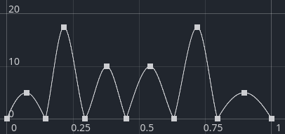
In between January and June, we’ll pretend that the weather parameters (temperature, precipitation) follow a sine curve. This isn’t actually too far from the truth, as you can see in these charts from a 1936 publication by Wladimir Köppen (who’ll show up again in a future post):
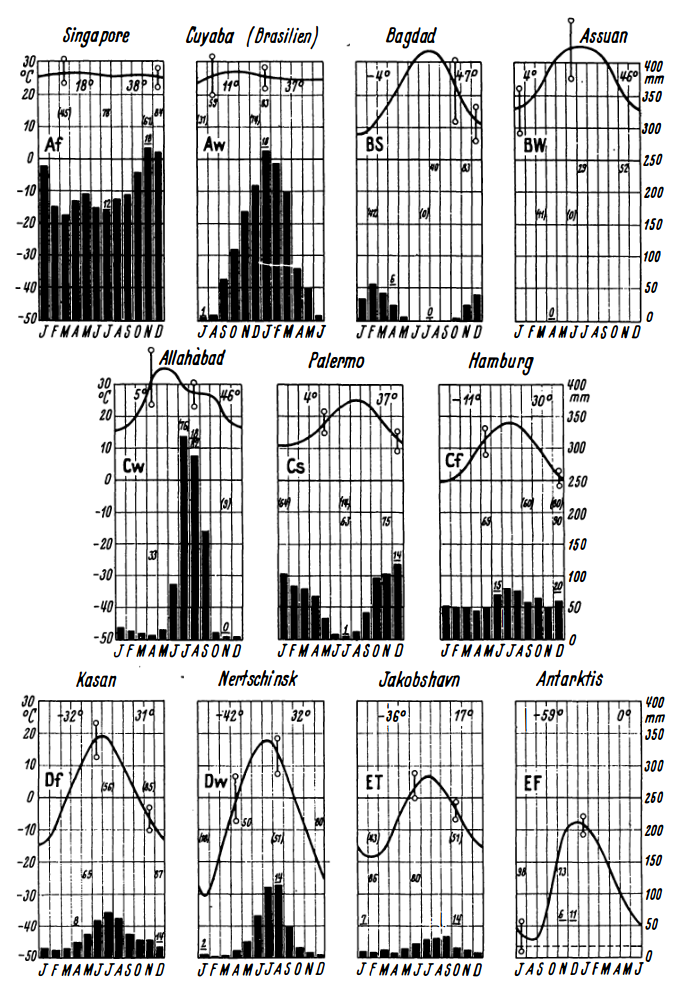
Source: Köppen, W. (1936) (PDF)
The wavy lines are the temperature, and the bars are precipitation. Both of these roughly follow a sine wave pattern in most cases.
Temperature
How do we get the weather for, say, January? Actually the algorithms are the same; only the input is different.
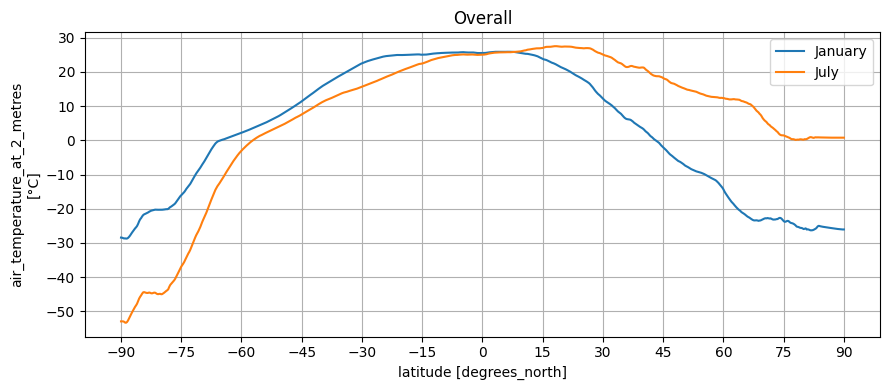
To start out with somewhat realistic values, let’s look at the real Earth first. I updated the notebook to split out the average temperature into a January and June part. In January the sun is above the southern hemisphere, so the temperature curve leans towards the negative latitudes, and in June it’s the reverse:
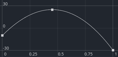
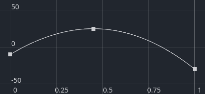
This translates to the following curve for January:
For June, the code simply mirrors this curve horizontally.
You might have noticed that the curves for Earth aren’t actually mirror images of each other; it’s considerably colder on the south pole (-90° latitude) than on the north pole (90° latitude). This is because of the influence of the sea, which reduces temperature differences between summer and winter.
This effect is quite significant. For example, winter in Antwerp, Belgium has an average temperature of 4.0 °C, whereas winter in Astana, Kazakhstan averages -14.5 °C. A difference of 18.5 °C, even though both are at 51° latitude! Similarly, summer in Antwerp is 18.9 °C on average, while it’s 20.6 °C in Astana. Not such a dramatic difference, but still.
The cause of this difference is that in winter, the wind coming in from the ocean is relatively warm, and in summer it’s relatively cool. So it seems we’re not going to be able to avoid blowing temperature around, in the same way we did with precipitation. But to give me some more control and improve performance, I’m doing it a bit differently: for each point, the algorithm traces the wind vector backwards, until it encounters sea. It calculates how many hours it took for the wind to reach that point from the sea, and based on that number it assigns a “continentality” factor between 0 and 1. Here’s what it looks like:
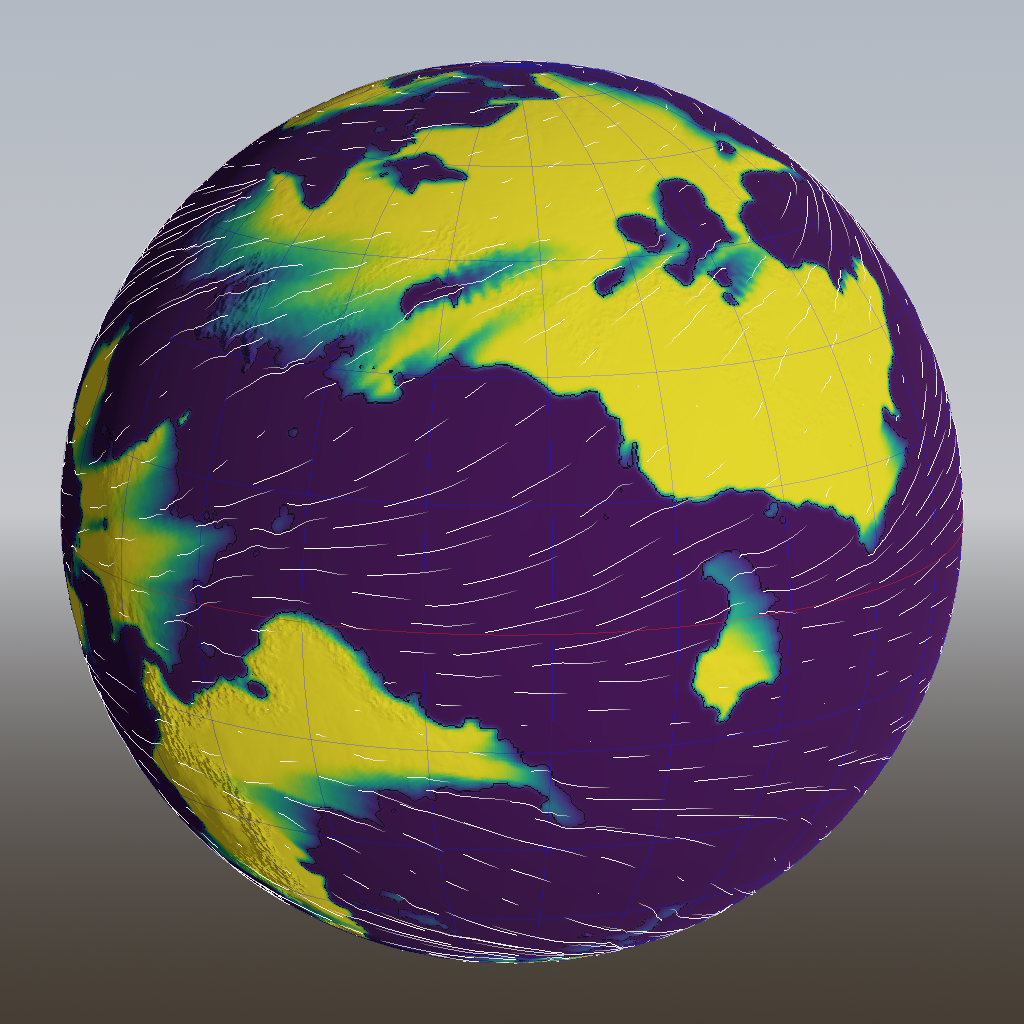
You can see how winds from the sea blow the low continentality further inland, but where the wind blows away from land, there’s quite a sharp transition.
Then I split the latitude-dependent temperature curve in two: one for oceanic, one for continental. The continentality factor is used to mix between them:
Oceanic temperature curve
Continental temperature curve
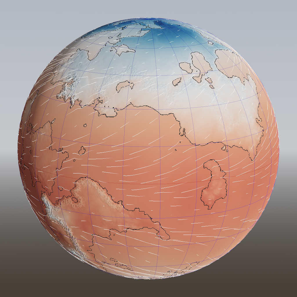
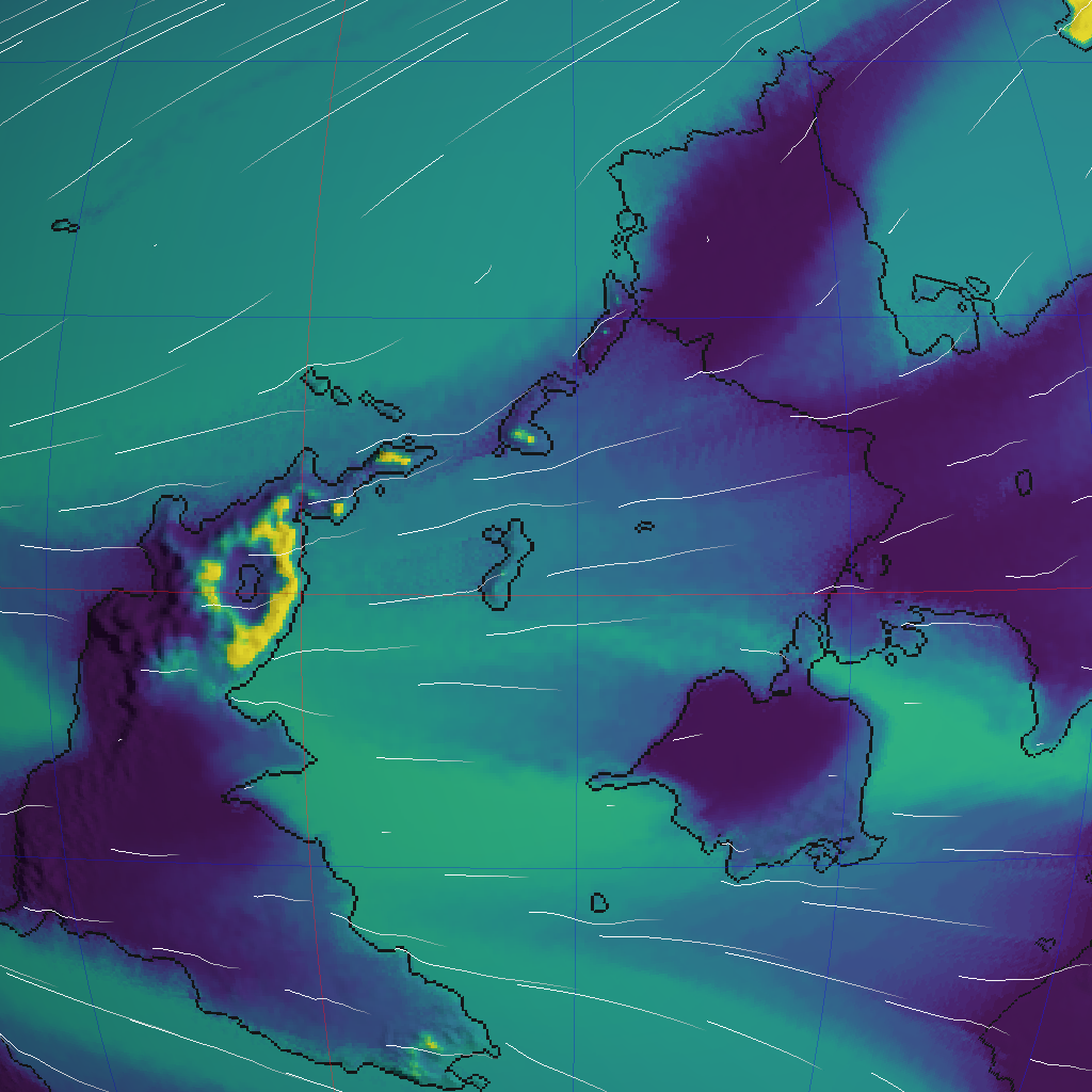
And that yields a temperature map where locations farther inland have more extreme temperatures, as is most clearly visible on the large northern continent:
Rain
Evaporation follows directly from temperature, so it doesn’t need any changes. Precipitation follows from evaporation, temperature and wind, so that’s covered too. We simply run the same rain propagition algorithm twice.
Simply.
However, remember the trouble I went through to make rain propagation (convection) fast enough to run it even one time. And now we have to do it two times?
Fortunately I have another trick up my sleeve. In the first few time steps of the rain propagation algorithm, there’s still a lot of moisture in the air, so it matters a lot where exactly it falls. But later on, when most of the rain has already been deposited, such precision matters less. We can make use of that: after 10 time steps, we downsample the map by a factor of 2, and run the remaining time steps at half the resolution. This saves 4× on data and thus running time, but it also allows us to get away with a time step twice as large.
Instead of 50 full-resolution time steps, we can just take 10 full-resolution steps and (50 - 10) / 2 = 20 half-resolution time steps. In both cases, about 97% of rain is dropped, but the original process takes 0.8 seconds whereas the new process takes only 0.25 seconds. Original version above, new one below:
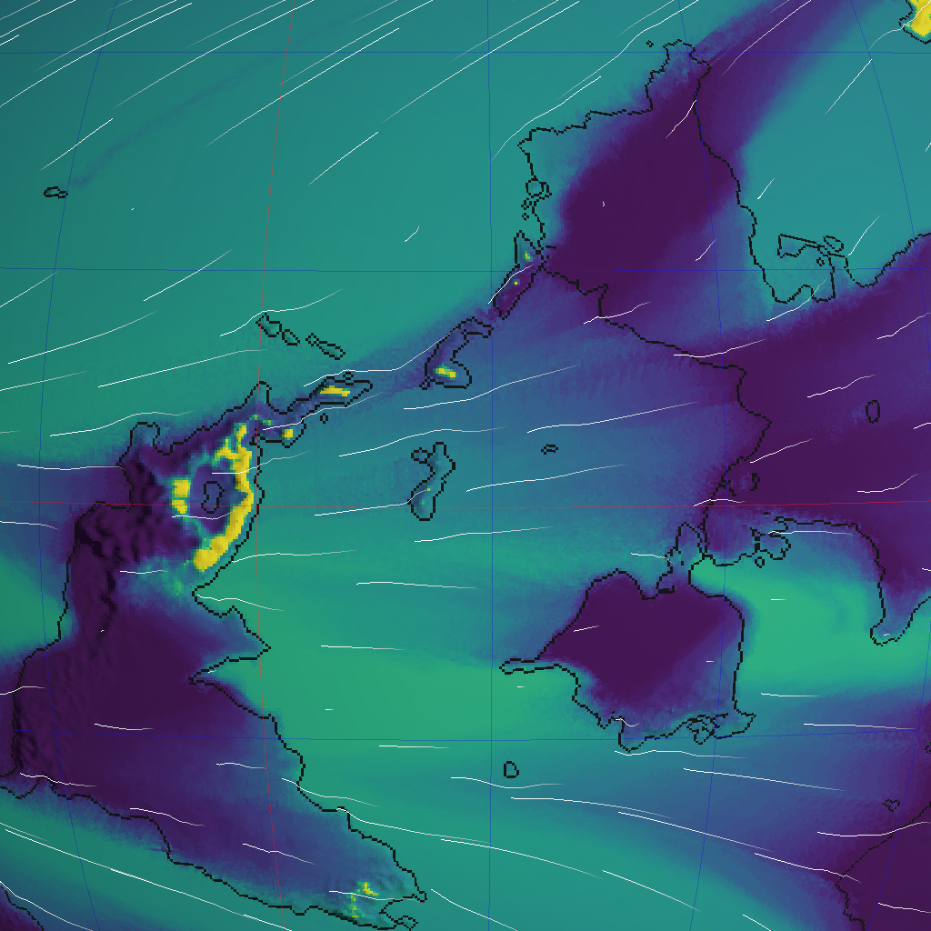
It looks a bit softer around the mountains, but overall the difference is negligible.
Wind
Wind does need some changes to introduce seasonality, because the ITCZ (inter-tropical convergence zone), which forms the boundary between the northern and southern Hadley cells, also follows the sun. Here’s how the wind speed on Earth depends on latitude:
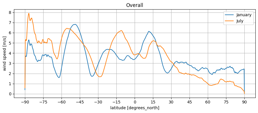
It’s a pretty messy pattern because of all those pesky continents, but you can see the effect of the Hadley cells as the two large bumps on either side of 0°. The trough between them is a bit north of the equator in July and south in January.
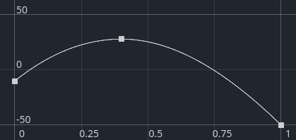
Trying to filter out the effects of landmasses, I guess that the idealized pattern in January ought to look something like this:
Again, the curve is mirrored for July. (Keen-eyed readers might notice that the scale on the y axis is different — the peaks in my curve are much higher than in the Earth plot above. This is because the plot is based on a convenient but quite incorrect approach to calculating wind speed: it averages over all the wind vectors, then computes the length of the average, instead of the other way round.)
Here’s an animation of the result; you can clearly see the ITCZ and horse latitudes moving north and south:
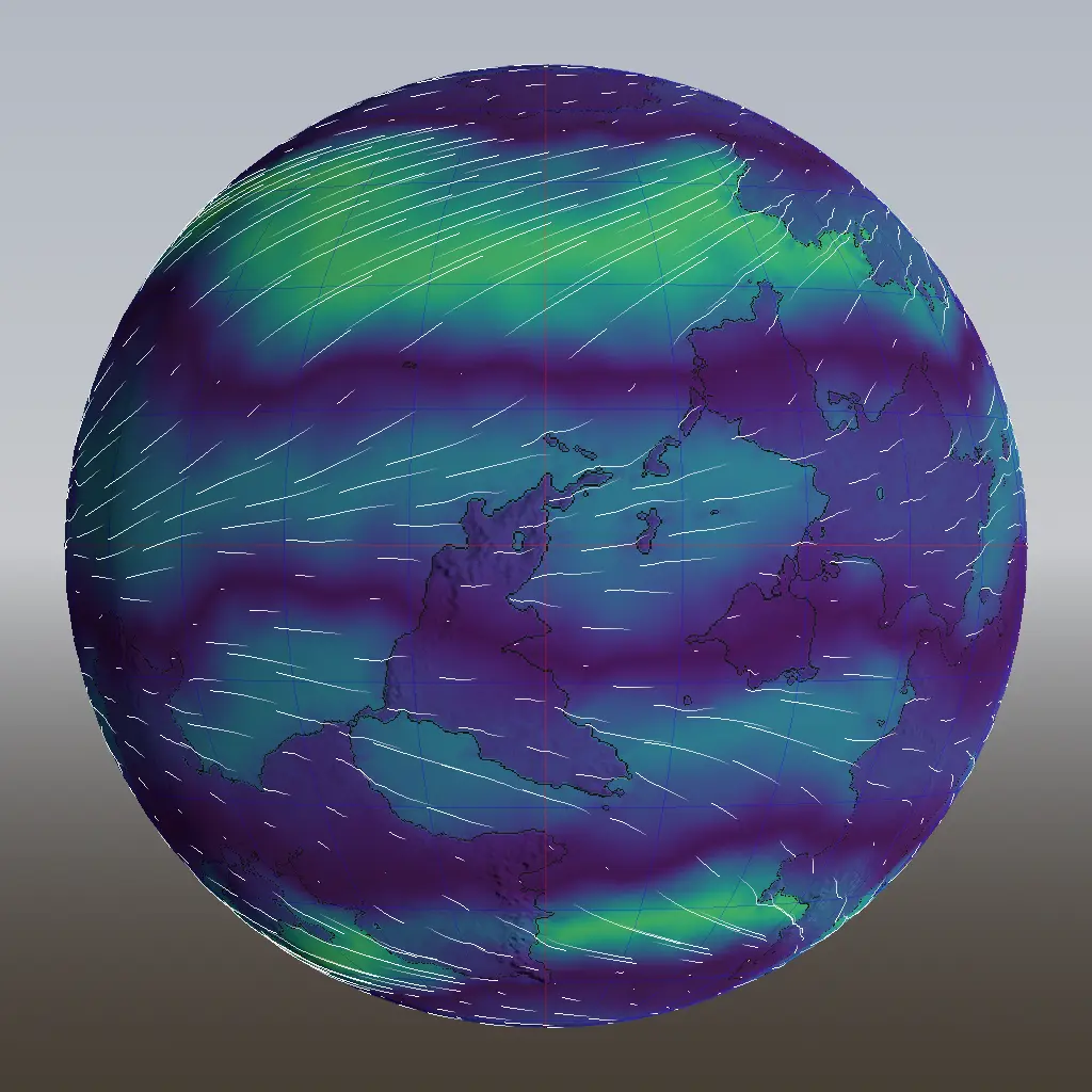
Regions between these moving boundaries will have a highly variable wind pattern, blowing from the east in one season and from the west in another. These are monsoon winds, so we got those for free!
Now what?
I had hoped that splitting the yearly weather in two, one for January and one for July, would be a simple matter of running the same code twice. It turned out to be a bit more work, but the results became more accurate and running time didn’t suffer. In the next post we’ll tackle climate classification, and we’ll see whether the effort has been worthwhile.