Around The World, Part 5: Wind pressure
This post is part of a series about Around The World, a game of exploration and discovery at sea. The game is currently in early development. If you're new to this project, you can read up on it here.
Last time, we got some basic wind patterns going. However, there’s still a problem.
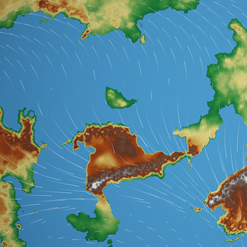
Looks alright, but sometimes this happens:
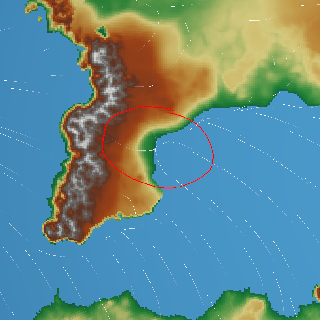
In the bay near the middle, streamlines from all different directions are converging to a single point. That means air is flowing to that point from all directions, but never leaving it again – that doesn’t seem very believable! And even if the player doesn’t notice the lack of realism, they would definitely notice that they aren’t able to sail out of that place.
In this post, I’ll describe a failed attempt to tackle this problem. It’s going to be somewhat heavy on maths and code, but we’ll be back to pretty screenshots soon, I promise.
Under pressure
In real life, this wouldn’t happen because the air pressure at that point would rise and push back against the incoming wind, which would be deflected away. But our simple blur is too naive to know about that effect.
In mathematical terms, we want the wind velocity’s vector field to be divergence free. In programming terms, this means that the amount of air flowing into each grid cell must be equal to the amount flowing out of it.
You might think that we can easily adjust the velocity in each grid cell so that the amount flowing in is equal to the amount flowing out. And yes, this is easy to do for one cell, but the change will cause the divergence in other cells to change. It’s an iterative process.
There is a mathematical theorem called Helmholtz decomposition, which states that each vector field (like our velocity field) can be written as the sum of a curl-free vector field and a divergence-free vector field. It’s the divergence-free part that we’re after. But how do we compute it?
At this point, I remembered my previous work (over 13 years ago!) on fluid simulation, and in particular a well-known article by Jos Stam. He describes a relatively simple C function which tackles exactly this problem of making a velocity field divergence free:
void project ( int N, float * u, float * v, float * p, float * div )
{
    int i, j, k;
    float h;
    h = 1.0/N;
    for ( i=1 ; i<=N ; i++ ) {
        for ( j=1 ; j<=N ; j++ ) {
            div[IX(i,j)] = -0.5*h*(u[IX(i+1,j)]-u[IX(i-1,j)]+
            v[IX(i,j+1)]-v[IX(i,j-1)]);
            p[IX(i,j)] = 0;
        }
    }
    for ( k=0 ; k<20 ; k++ ) {
        for ( i=1 ; i<=N ; i++ ) {
            for ( j=1 ; j<=N ; j++ ) {
                p[IX(i,j)] = (div[IX(i,j)]+p[IX(i-1,j)]+p[IX(i+1,j)]+
                p[IX(i,j-1)]+p[IX(i,j+1)])/4;
            }
        }
    }
    for ( i=1 ; i<=N ; i++ ) {
        for ( j=1 ; j<=N ; j++ ) {
            u[IX(i,j)] -= 0.5*(p[IX(i+1,j)]-p[IX(i-1,j)])/h;
            v[IX(i,j)] -= 0.5*(p[IX(i,j+1)]-p[IX(i,j-1)])/h;
        }
    }
}
I’m not going through this in detail, but you can see that there are three parts here, each consisting of some nested for loops. (I’ve removed the set_bnd calls because a spherical surface conveniently has no boundaries.)
The first part computes the divergence (called div) in each grid cell. Actually, I think it’s the negative divergence here; we could call it convergence.
The second part computes the pressure (called p) in each grid cell, which would result from this divergence. It does by solving a simple differential equation through an iterative process called Gauss-Seidel iteration. This will gradually converge towards the exact solution; Stam cuts it off after 20 iterations.
The third part computes the gradient of the pressure, and applies it to the velocity (whose x and y components are called u and v), which should result in a divergence-free velocity field.
Insanity laughs
This is easy to formulate on a square grid, but more difficult on a sphere. Remember that I’m using a cube grid that has been projected onto the sphere. Consider, for example, the red cell in the corner of the top face (which covers the north pole):
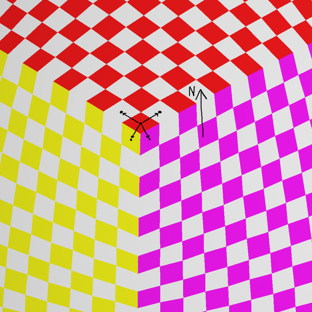
The edges of that square don’t align neatly with the compass directions, but are rotated a full 45° so that global north actually points to a corner of the cell. To add to the difficulty, the cell’s left and right neighbours aren’t even straight opposite each other, nor its top and bottom ones.
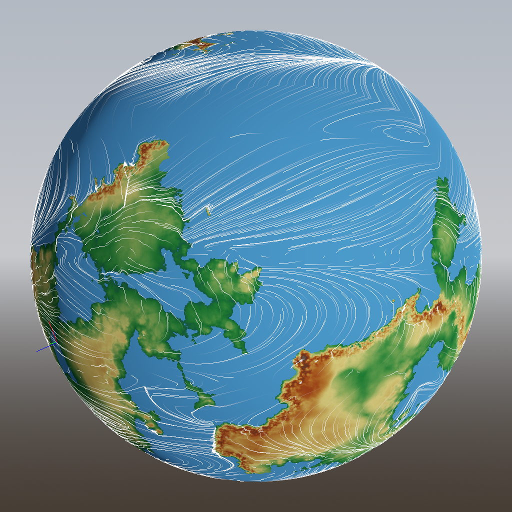
To make this work, I tried to express everything in the cell’s local coordinate system, even though its x and y axes are not usually orthogonal. However, this results in sudden changes in the pressure gradient, which I wasn’t able to get rid of, as you can see in the northern hemisphere where the wind turns sharply around a corner:
I tried other coordinate axes, but they had similar issues.
And that isn’t the end of the problems with this approach. Despite using 10000 iterations to allow the pressure to converge, there are still sharp transitions, as you can see next to the mountain range in the south where the wind just seems to bounce off rather than bending sideways gradually.
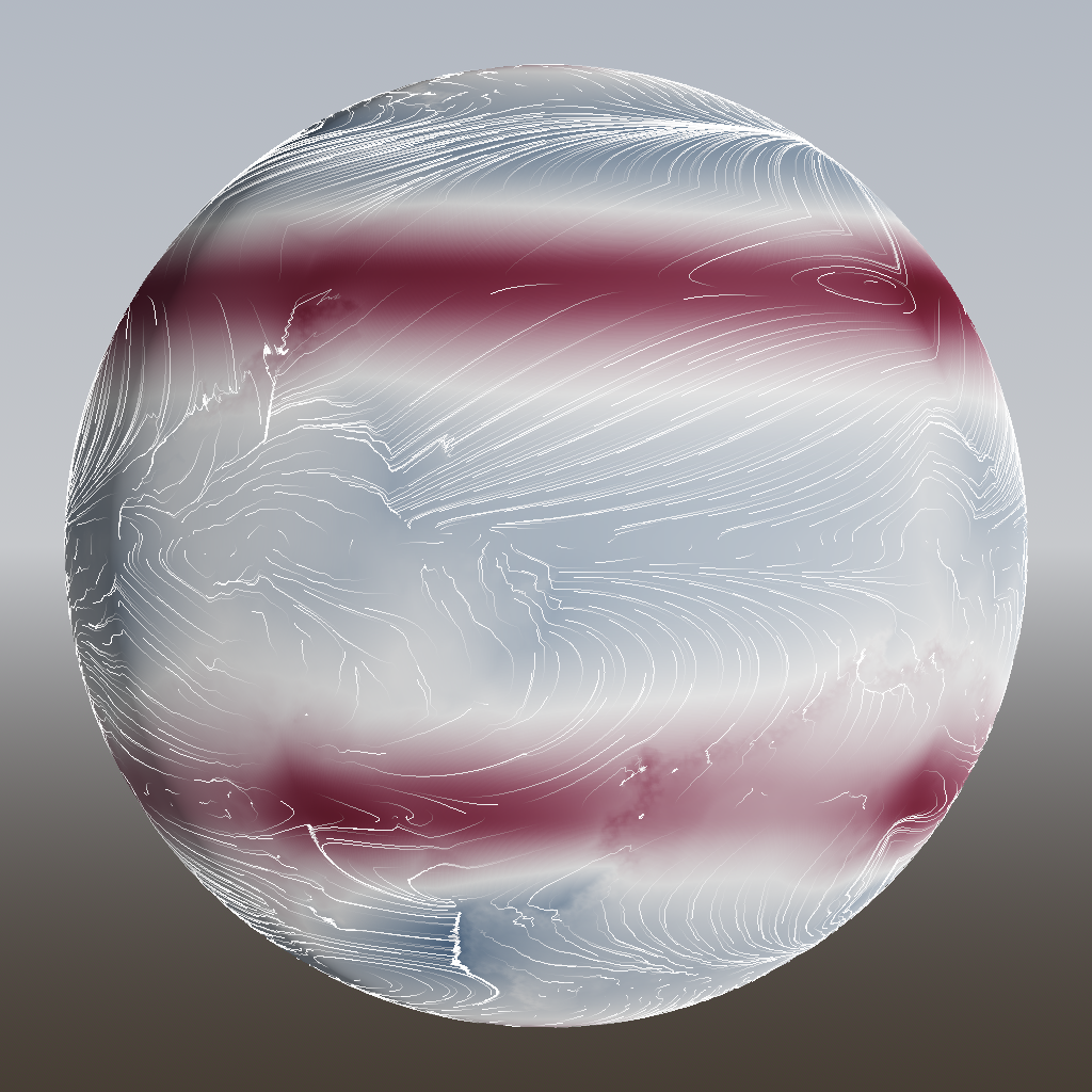
But it gets worse. Remember that I added bands at 0°, 30° and 60° of latitude to serve as “sources” and “sinks” of wind. These have nonzero divergence too, and they should, because air does appear and disappear here (from and to higher layers of the atmosphere). But the pressure solver doesn’t know that, and tries to correct for it, resulting in these bands:
On top of all that, running 10000 iterations takes about 4 minutes, which is much too long. I’m aiming to have the entire world generation run in at most 5 seconds on my fast computer, so that people on slower computers can still play the game too. There are many ways to speed it up:
- ~4×: Use an alternative algorithm which converges faster, such as SOR (successive over-relaxation) with a checkerboard update scheme.
- 4×: Parallelize better. Right now, I’m running one thread for each cube face, resulting in a 6-fold speedup, but my computer has 24 cores.
- 8×: Run at half the resolution. Not only do we have to do 4× less work, but convergence should also be at least 2× faster.
- ~10×?: Run it on the GPU, using Godot’s new experimental support for compute shaders.
Multiplying this all together gives us a speedup of over 1000×, more than enough to make this algorithm run quickly. But that won’t solve any of the other, more fundamental problems.
Moreover, this physics-based approach also means I’m giving up some control over how the wind patterns turn out. And considering how important wind is to the game, that might not be a good idea.
Back to the drawing board.