Around The World, Part 11: Everything is harder on a sphere
This post is part of a series about Around The World, a game of exploration and discovery at sea. The game is currently in early development. If you're new to this project, you can read up on it here.
I didn’t have time during the holidays to implement any new features, so enjoy this filler post that I prepared earlier! In the very first post in this series, I wrote:
The prototype took place on a rectangular map, with the left side wrapping around to the right to form a cylinder. […] Many games do this and get away with it, but because I’m a perfectionist, I want my game to take place on an actual sphere.
Today I’m going to write up in some detail why spheres are harder to work with.
Coordinates are harder on a sphere
Simply identifying a point on a sphere sounds like it should be easy, right? Isn’t that what spherical coordinates are for? You simply use phi and theta, or latitude and longitude.
And yes, that works for identifying points. But it’s a terrible system to do any kind of operations with. How do you compute the distance between two lat/lon pairs? How do you rotate from one point to another? And so on.
Fortunately, there’s a better way: unit vectors. Instead of identifying a point with two coordinates (x, y), we use three: (x, y, z). This is a regular 3-dimensional vector, but we require that it’s a unit vector, i.e. it has a length of 1. It wastes some memory, but it makes up for it in ease of operations, as we’ll see.
Think of this vector as an arrow, pointing from the centre of the sphere to a point on the sphere’s surface. Alternatively, you can think of it as just a point in 3D space, which is on the surface if you assume that the sphere is a unit sphere (i.e. a sphere of radius 1).
Geometry is harder on a sphere
Fortunately, once we have settled on 3-vectors to identify points, geometry on a sphere isn’t that much harder than on a plane. It just requires more thinking.
For example, a distance in the plane is easy to calculate using the Pythagorean theorem. On a unit sphere, the distance between a and b is actually just the angle between the two unit vectors. This is easy to compute as acos(dot(a, b)).
What about movement? In a plane, we represent a velocity as another (vx, vy) pair, which represents a translation. On a sphere, like with points, we could just represent a velocity as a vector (vx, vy, vz). The trouble with that is that, after you add it to some point, the point is no longer a unit vector, and reprojecting it back onto the unit sphere loses some of the velocity. So we’ll have to come up with something better.
We can also model a velocity as a rotation around the centre of the sphere. A rotation can be represented as a 3×3 matrix, or more compactly as a unit quaternion. However, not every rotation is a plain translation along the surface; it may also have a rotational component around the point itself. Imagine yourself taking a step forwards, but pivoting to face to your right at the same time. So a better equivalent of a 2D translation would be “a rotation around an axis through the centre of the sphere which is perpendicular to the point being translated”.
A pair of two numbers also works: one to represent the absolute speed, and the other the compass bearing. This is similar to polar coordinates. I’m using this as the initial representation of wind velocity because it’s what comes out of my parameters, but then immediately convert it to a 3-vector so I can do math to it.
So we can work with points, but what about lines? A straight line on the plane is infinite, but on the sphere, it bites itself in the tail and becomes a great circle instead. We can represent such a circle as yet another unit vector, pointing orthogonal to the circle.
Grids are harder on a sphere
By and large, game worlds come in two flavours: meshes and grids. First-person 3D games typically use free-form meshes, but most games with a top-down perspective are based on some kind of grid.
On a plane, grids are easy. A grid of squares is the most natural and straightforward to work with. Isometric grids have diamond-shaped cells, which are just distorted squares. Hexagons are a step up from there, but they’re well documented by the awesome Red Blob Games.
On a sphere though, none of these approaches work. We can take a 2D grid and try to map it to a sphere somehow. The simplest way to do that is the equirectangular projection, a.k.a. plate carrée projection, where x becomes longitude and y becomes latitude:
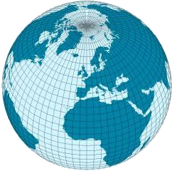
Source: Wikimedia Commons by Stefan Kühn, CC-BY-SA 3.0
But none of the squares actually end up as squares, those at the equator are much larger than those near the poles, and the “squares” directly at the poles are actually triangles! This is problematic if we want to run any kind of simulation on there, because those usually need grid cells of (approximately) the same area.
We can obtain a grid with less distortion by starting out with one of the five platonic solids as a base shape:
| Tetrahedron | Hexahedron | Octahedron | Dodecahedron | Icosahedron |
|---|---|---|---|---|
 |  |  |  |  |
Image source: Wikipedia by DTR, CC-BY-SA 3.0
Then we subdivide each face and project the new points outwards onto a sphere.
Which platonic solid do we pick? The dodecahedron is out of the question; pentagonal faces can’t be subdivided into smaller regular pentagons. There are three solids with triangular faces: the tetrahedron, octahedron and icosahedron. For the minimum amount of distortion, it makes sense to start with the icosahedron, because it has the closest resemblance to a sphere already. A subdivided icosahedron looks like this:
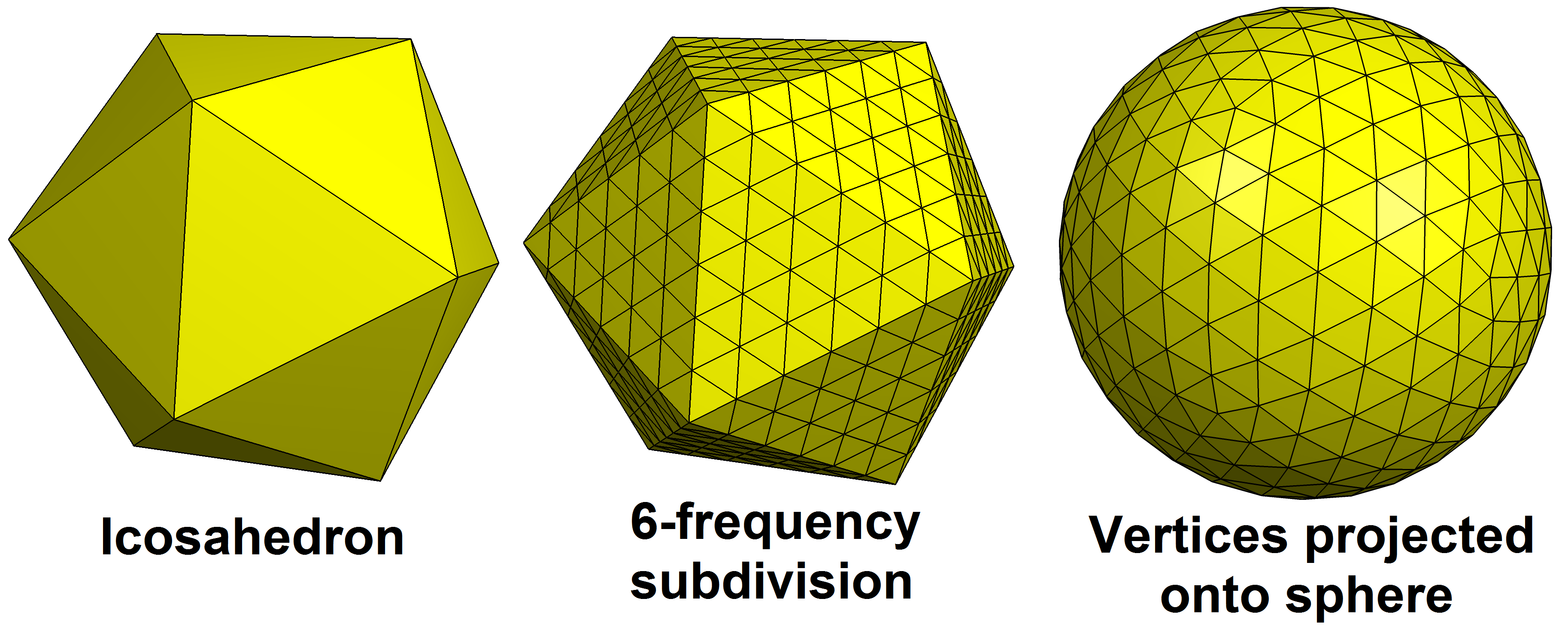
Source: Wikimedia Commons by Tomruen, CC-BY-SA 4.0
It’s looking great with very little distortion, but the drawback is that triangular grids are harder to work with than square grids. For example, they don’t map to a 2D array or a texture as easily as a square grid does.
That leaves the hexahedron, popularly known as the cube. This is what I ended up with, as explained in the first post. But the subdivided icosahedron might make a comeback once we start building meshes!
Areas are harder on a sphere
On a truly regular grid, we can compute areas simply by counting grid cells. Our quad sphere isn’t truly regular though, so whenever we want to compute an area, we have to compensate for each grid cell’s area.
This is used in my code, for example, to adjust the water level so that 71% of the world is water.
Neighbours are harder on a sphere
Neighbour lookups are used a lot in my code, for example to compute gradients, find tectonic plate boundaries, and perform various flood fill operations.
In a regular square grid, the four neighbours of a grid cell are easy to find: x+1, x-1, y+1, y-1. But because our grid isn’t exactly regular, it becomes more difficult. Within each cube face, the approach still works, but as soon as we have to wrap around to another face, we have to juggle all the coordinates around to find the right grid cell in the adjacent face. I use this mapping, which has a pattern to it that makes the math slightly easier:
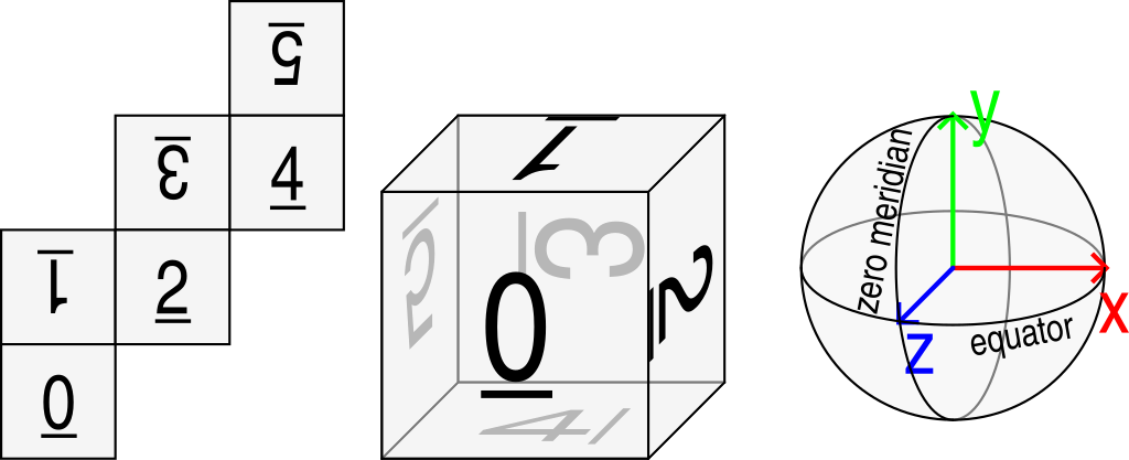
The pattern is that, whenever you cross an edge, the coordinate axis parallel to that edge always flips. For example, if you go off the top of face 0 into face 1, the x axis flips, and if you go off the right of face 0 into face 2, the y axis flips (and also becomes the x axis). Because of the regularity of the face numbering, you can also do some modulo tricks to reduce the number of if statements needed.
An alternative (shout-out to acko.net) is to “dilate” each cube face, essentially adding another strip of grid cells around it that’s just a copy of the cells from the adjacent face. Then you don’t ever need to wrap to another cube face, because you can simply go 1 cell out of bounds and find the value there. This is nice for read-only operations, but e.g. flood fills still require that you actually wrap around to the adjacent face.
Interpolation is harder on a sphere
In the grid defined by our quad cube, cell values are theoretically defined at the cell’s centre. So what if we want to compute the value at some other point, that isn’t exactly in the middle of a cell? This is needed, e.g., for the backwards advection of rain along the wind vector field, mentioned previously. The answer is: interpolation.
In a 2D square grid, this would be a straightforward bilinear interpolation. It’s so straightforward even, that GPUs implement it in hardware.

Source: Wikimedia Commons by Swienegel, CC-BY-SA 4.0
Suppose the Q’s are our grid cell centers. First we interpolate between Q11 and Q21 to find the value at R1, and between Q12 and Q22 to find the value at R2. Then we interpolate between R1 and R2 to find the desired value at P.
On the quad sphere though, we don’t only have to account for wrapping to another cube face (like with finding neighbours), but also with differences in distance because due to distortion, some neighbours are closer than others.
Noise functions are harder on a sphere
I’ve mentioned simplex noise several times on this blog. I haven’t mentioned that all simplex noise that I’m using is 3D. Technically it exists not only on the sphere’s surface, but also inside and outside it. This is the easiest way to get continuous noise on a sphere with (virtually) no distortion.
Since simplex noise is based on a triangle grid, I considered building my own simplex noise algorithm based on a subdivided icosahedron, something I haven’t seen done anywhere before. It might speed up noise generation more than twofold, because time complexity of n-dimensional simplex noise scales as n². But 3D is fast enough for me in practice, so I didn’t bother.
Splatting is harder on a sphere
By “splatting” I mean: drawing a sprite of some small maximum radius onto the map. This is used to create volcanic islands caused by hotspots.
On a 2D grid, we could just find the square bounding box of the sprite and loop over all the cells in the bounding box. But on the sphere, such a bounding box is (a) much harder to compute, and (b) not a box.
So what I’m doing instead is a Dijkstra flood-fill algorithm, which starts from the centre and terminates when the maximum radius has been reached. This is far less efficient, but for small areas it doesn’t matter.
Distance transforms are harder on a sphere
The distance transform of a grid of booleans (0/1) gives, for every cell whose value is 0, the distance to the nearest cell whose value is 1. This is useful, for example, to apply effects whose strength depends on the distance to the coast, or to a tectonic boundary.
It’s surprisingly difficult to compute the distance transform efficiently. In square 2D grids, the state of the art is an algorithm by my former professors Meijster, Roerdink and Hesselink: A General Algorithm for Computing Distance Transforms in Linear Time. It’s easy to implement, but only works on square grids.
Instead, I used a similar trick as with splatting: starting from all points on the boundary simultaneously, perform a multi-source Dijkstra flood fill until all cells have been visited and annotated with their distance. This is relatively slow due to all the random memory access, does not parallelize well to multiple CPU cores, and has edge cases where it doesn’t give the exact distance transform – but it’s just barely good enough for my purposes. (The slowest parts of the world generation are those using this algorithm or some variation of it.)
Worth it?
I’m sure the above list is not exhaustive. At least two things are coming down the pipeline which are also harder on a sphere: spatial indexing, and physics. So maybe there will be a Part 2 to this post at some point.
Should I have copped out and made the world a cylinder instead? Maybe. But I’m hoping that by taking place on an actual sphere, the game might appeal more to map nerds (we need to do map projections!), and generally stand out a little bit more in the crowded indie games market. Time will tell.